Data Assignment #3 (due March 30, 2025 by 11:59pm)

As we come to the end of the term, our last two topics are electricity and climate change and this data assignment combines both of those subjects. I also want you to work towards being able to present really nice-looking markdown html documents including the suppression of some of the code, warnings, etc. from your final document. As such, part of the requirements for this exercise are for you to make use of chunk options for your r code to improve your presentation of data. We’ll also use cached data so that you don’t have to re-download data every time.

For this data assignment, you’re going to use a few different sources of data:

Canada’s Greenhouse Gas Emissions Projections;
Canada’s National Greenhouse Gas Emissions Inventory; and
AESO merit order data (the supply curve!).

There’s a challenge graph with a couple of new skills for you to master!

Are you ready to get started?

Make sure you read all the instructions closely and make sure to comment your code and only add a bit at a time to your RMD files so that you can easily spot errors or the impacts of changes you’ve made.

To execute the output you see below, I’ve used the following packages. Use this as a guide to set up your document:

#usual packages
library(readxl)
library(janitor)
library(tidyverse)
library(lubridate)
library(scales)
library(viridis)
library(cowplot) 
library(ggthemes)

theme_ps <- function() {
  theme_cowplot() + 
    theme(
      text = element_text(size = 12, color = "black"), 
      plot.title = element_text(size = 14, face = "bold", hjust = 0.5),
      axis.title = element_text(size = 12, face = "bold"),
      axis.text = element_text(size = 11), 
      axis.line = element_line(color = "black", size = 0.8),
      panel.grid.major = element_blank(),
      panel.grid.minor = element_blank(),
      legend.position = "bottom", 
      legend.title = element_blank(),
      legend.text = element_text(size = 11)
    ) + 
    theme(plot.margin = unit(c(1,1,1,1), "cm"))
}

You may find it useful to have another look at the Functions Demo before you start this assignment.

A lot of the plots in here rely on different ways to order data stored as factors. Remember way back from the first data exercise, we looked at factors and a package called forcats that lets you manipulate factors. We’re going to use this package in a couple of spots in this assignment.

Deliverable 1: Cleaning up your html (1 total mark)

The first thing I want to see from you this time is cleaner html files. I want you to use chunk options to set up your output to look much cleaner in the html you generate. You’ll want to have this explainer on chunk options and this more detailed version to hand. For default settings in my code, I include the following chunk right at the top of my document. Setting warnings and messages to false means that you don’t get all the red text mirrored into your html (you might want to give that first chunk {r chunk_opts,include=F} options to suppress the output.

knitr::opts_chunk$set(message=F,
                      warning=F)#turn off messages and warnings
options(scipen = 999) #suppress scientific notation

For individual chunks in my code, I use echo=FALSE when I don’t want to show you the code, and include = TRUE when I want to show you both code and output.

If you want to try something a little more fun, try code-folding in your html which lets you create little radio buttons to show or hide your code (you’ve seen me use this in a few things this term, like this document).

Another useful thing you can use for code chunks is caching. If, for example, you have a code chunk that downloads data, cache that chunk using cache=TRUE in the chunk options and everything will run more quickly as you don’t have to download the data each time. You don’t have to do this, but you might want to know it’s an option.

And, finally, remember that you can use chunk options to modify figures. For example, chunk options as follows {r,out.width="95%",dpi=150,fig.align="center",fig.height=8,fig.width=14} will set the width of the graph window, the resolution (dpi), the alignment and the dimensions of the figure you’re pushing into your html. Make sure your figures look good in your final html!

With all of this in hand, you should be able to make a nice, efficient html file! I’d like you to try just to show me the code you use in the assignment, but to suppress warnings and messages from the final product and to make sure all figures clear and complete in the html. (1 mark)

Deliverable 2: Electricity Generation by Source, Canada (3 total marks)

Canada’s official Greenhouse Gas Emissions Inventory, the emissions against which our national targets are measured, contains data on electricity generation, and it’s some of the best data we have at a national level. From the homepage, you should navigate to the open data site and download the electricity data by province (it should be one large excel file).

If you look at the Excel file, you’ll see that it has a worksheet for Canada and for each province. You’ll also see that you need to do some data cleaning, which you can do in R to get the data you need, or you can do the manipulation in Excel and read in only the data to make this graph and the next one.

The first graph I’d like you to produce is one for Canada (2 marks).

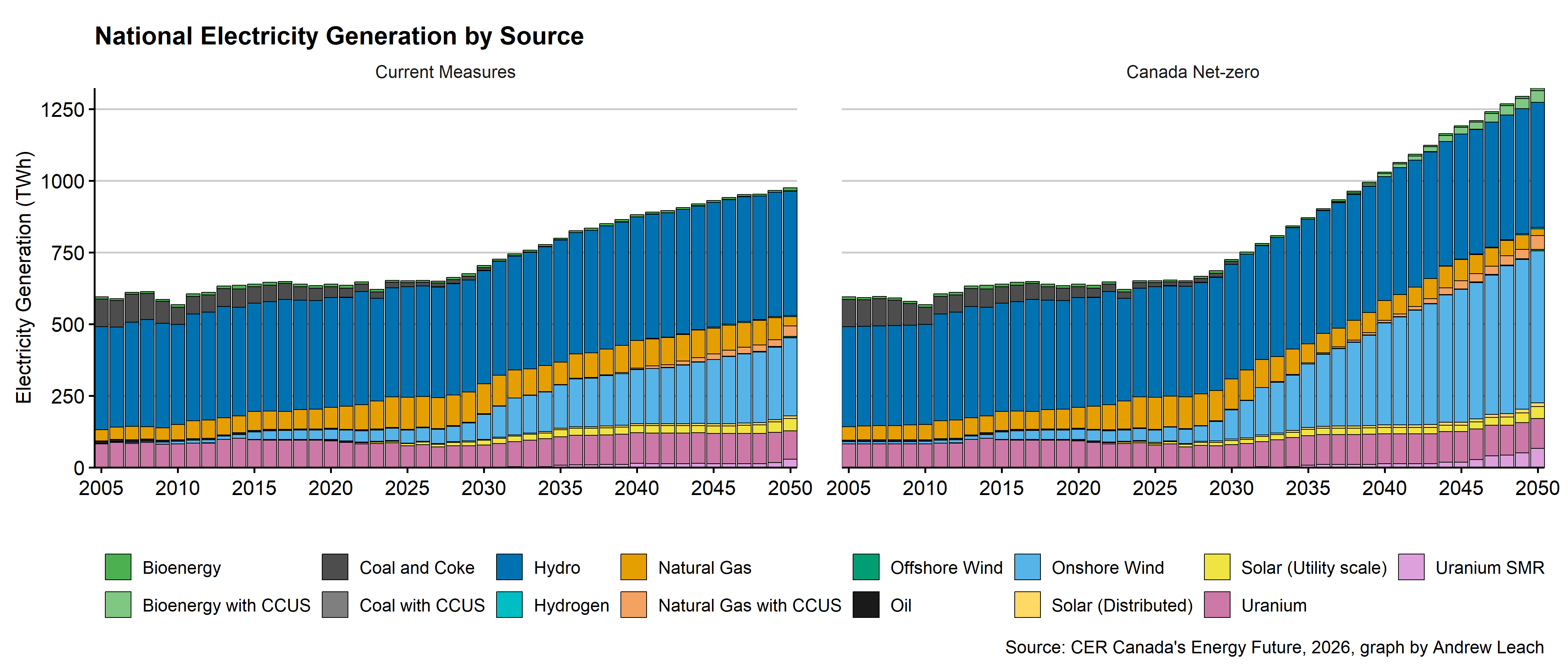
Your graph doesn’t have to be a perfect replication of this, but it should be similar. You’ll notice a few things from this graph: the data are not in an even sequence by year, and I’ve converted the data from GWh to TWh.

A couple of hints:

use year as a factor (i.e. use as_factor(year) after you’ve converted the data into long form using pivot_longer) and then graph using the factor as your x axis. You will NOT be able to make this graph with scale_x_date, so don’t even try. You don’t have even intervals between years, so use factors and scale_x_discrete to make some changes if you need to do so;
use geom_col() the same way you would use geom_area();
instead of using value in your graph, use value/1000 and you’ll get the different units;
if you’re getting scientific notation, add a line options(scipen=999) earlier in your r code;
if you want to tilt the x-axis labels, use theme(axis.text.x=element_text(angle=45,vjust=1,hjust=1)).

As a second deliverable in this section, I’d also like you to produce a similar graph for Alberta (1 mark).

Deliverable 3: Emissions from electricity generation (3 total marks, + 1 bonus mark available)

We’re going to talk a lot about emissions in the next while, so why don’t we get started now. Let’s look at how greenhouse gas emissions from electricity have evolved over time and by province. For this, we’ll use some data that we’re going to use a lot over the next couple of weeks: emissions inventories and data from Canada’s Fifth Biennial Report to the United Nations. Getting these data into R is a bit of a pain, so I’ll give you the data for this one in assignment_3_projections.csv.

If you want to see how I actually made these data for you, I’ve left the code in here (folded) for your reference.

Code

#Environment Canada Emissions Projection Data
file_loc<-"https://data-donnees.az.ec.gc.ca/api/file?path=/substances/monitor/canada-s-greenhouse-gas-emissions-projections/Current-Projections-Actuelles/GHG-GES/detailed_GHG_emissions_GES_detaillees.csv"
download.file(file_loc,destfile="ec_projections_2023.csv",mode = "wb")

#2023 Projections Data
proj_data<-read.csv("ec_projections_2023.csv",skip = 0,na = "-",fileEncoding = "Latin1", check.names = F) %>% 
  clean_names()%>%select(-c(2,4,6,8,10,12,14)) %>% #take out the french data
  pivot_longer(-c(1:7),names_to = "year",values_to = "emissions")%>% #switch to long form
  mutate(year=gsub("x","",year),emissions=gsub("-","0",emissions),year=as.numeric(year),emissions=as.numeric(emissions))
#clean the emissions data and the naming of the years

#reset names
names(proj_data)<-c("region","scenario","sector","subsector_level_1","subsector_level_2","subsector_level_3","unit","year","emissions")

#recode provinces
proj_data<-proj_data %>% filter(sector %in% c("Electricity"))%>%
  mutate(prov=as.factor(region),
         prov=fct_recode(prov,"AB"="Alberta",
                         "BC"="British Columbia",
                         "NL"="Newfoundland and Labrador",
                         "MB"="Manitoba",
                         "SK"="Saskatchewan",
                         "NS"="Nova Scotia",
                         "ON"="Ontario",
                         "NT"="Northwest Territory",
                         "NT"="Northwest Territories",
                         "QC"="Quebec",
                         "NU"="Nunavut",
                         "NB"="New Brunswick",
                         "YT"="Yukon Territory",
                         "YT"="Yukon",
                         "PE"="Prince Edward Island",
                         "NU"="Nunavut"
         ), #group the territories and the atlantic provinces
         prov=fct_collapse(prov,
                           "TERR" = c("NT", "NU","YT","NT & NU")
                           ,"ATL" = c("NL", "NB","NS","PE")
                           #,"OTHER ATL" = c("NL", "NB","PE")
         ))%>% #sum up emissions within territories and atlantic provinces
  select(year,prov,region,scenario,emissions,sector)%>% group_by(year,prov,sector,scenario)%>%summarize(emissions=sum(emissions,na.rm = T)) %>%ungroup()%>%filter(prov!="TERR") #drop the territories here



write.csv(proj_data,"assignment_3_projections.csv",row.names = FALSE)

These data are in a format you’ll be used to seeing: a reference case and an additional scenario, and they also contain historic emissions inventory data in the NIR2024 scenario. In order to keep the provinces in order from west to east, I’d suggest you use something like this in your code to format your provinces into a factor with labels in order:

proj_data<-proj_data %>% #reorder factor levels
  mutate(prov=factor(prov, 
                     levels=c("Canada" ,"BC","AB" ,"SK","MB", "ON","QC","ATL","TERR"  )))

You can also do this with fct_relevel from forcats:

proj_data<-proj_data %>% #reorder factor levels
  mutate(prov=fct_relevel(prov,"Canada","BC","AB" ,"SK","MB", "ON","QC","ATL","TERR"))

I’d like you to make a couple of different graphs using these data.

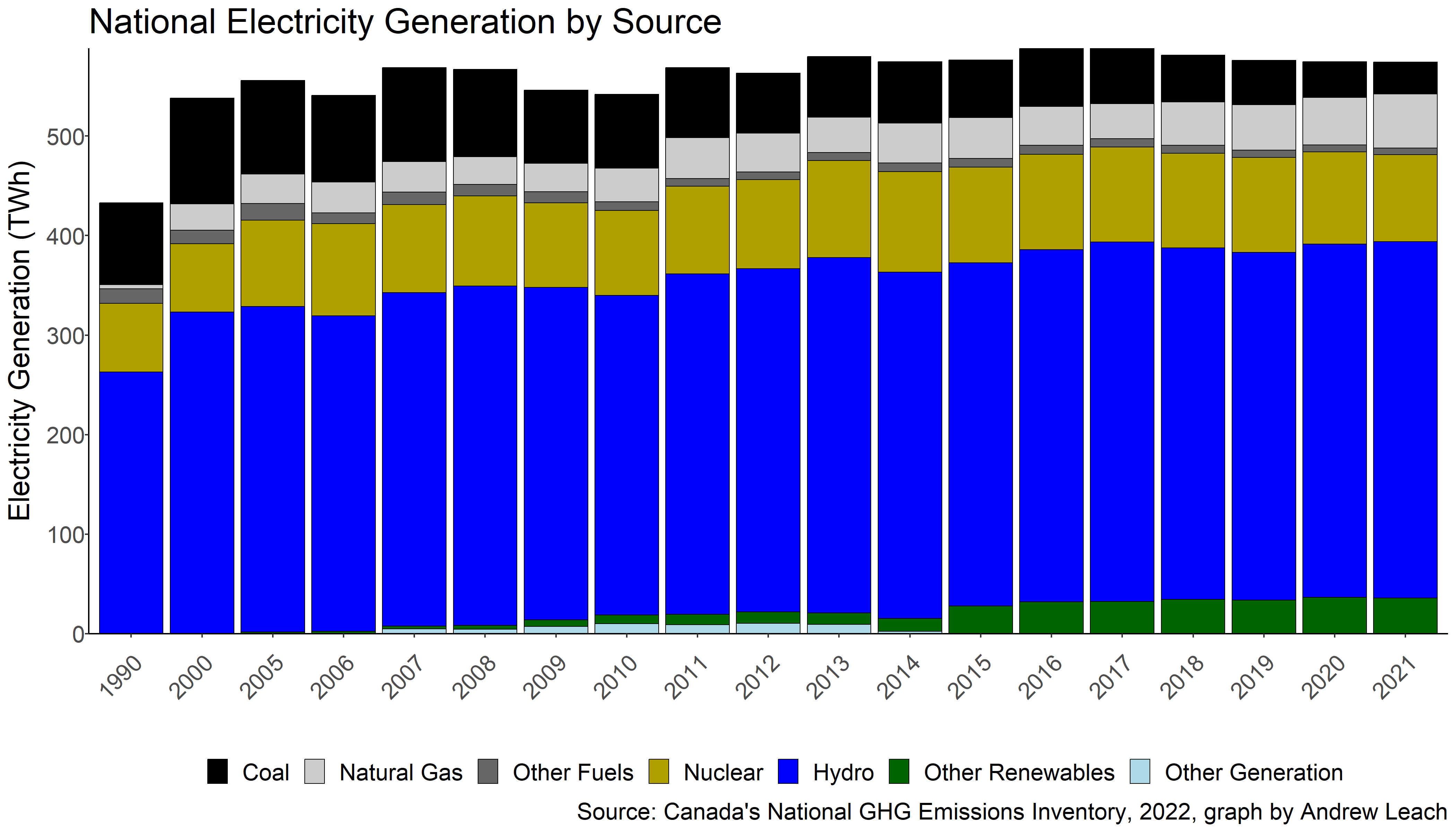
First, I’d like you to graph national emissions stacked by province, using the national inventory (NIR 2024) data from the file (1 mark):

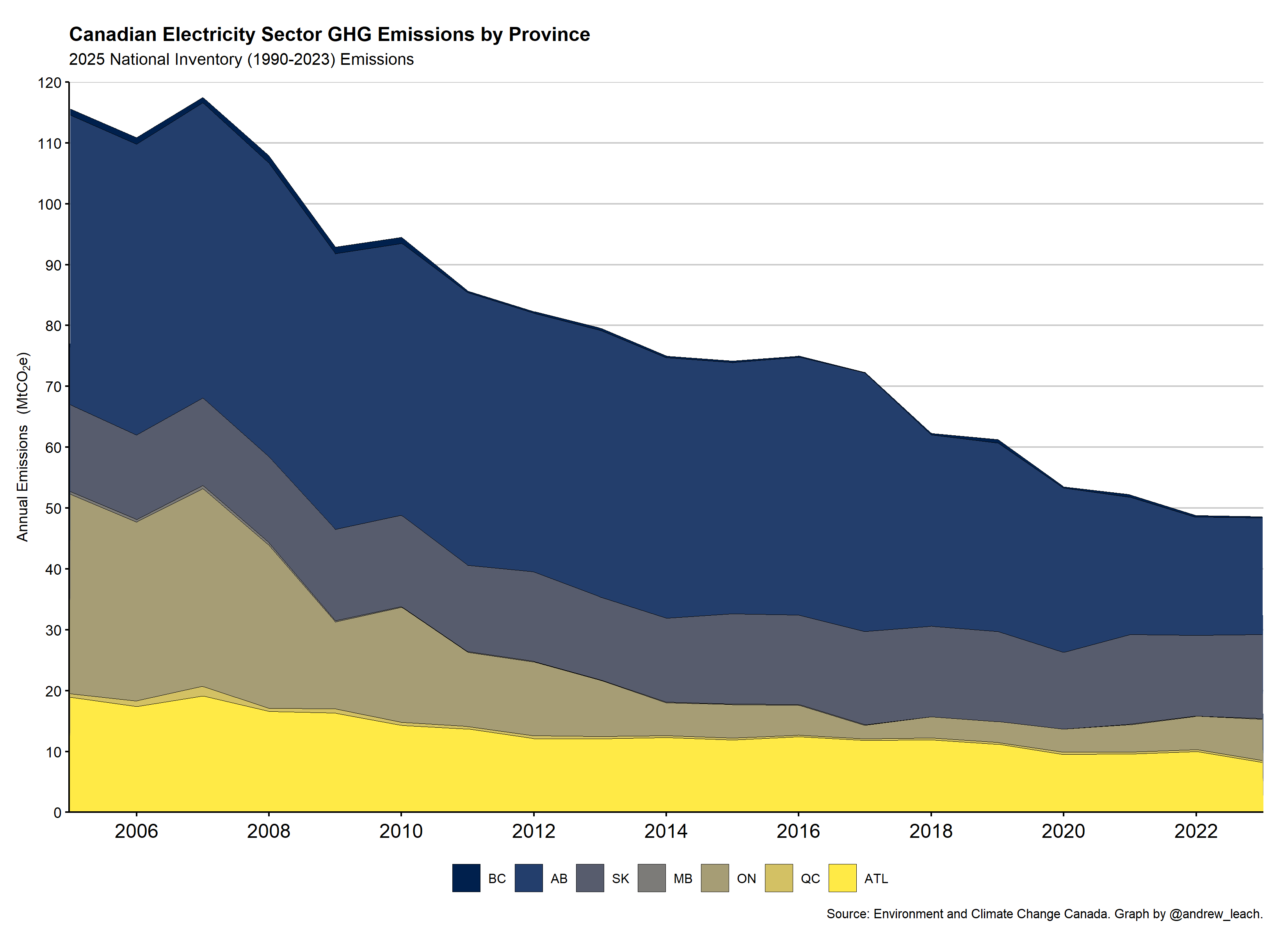
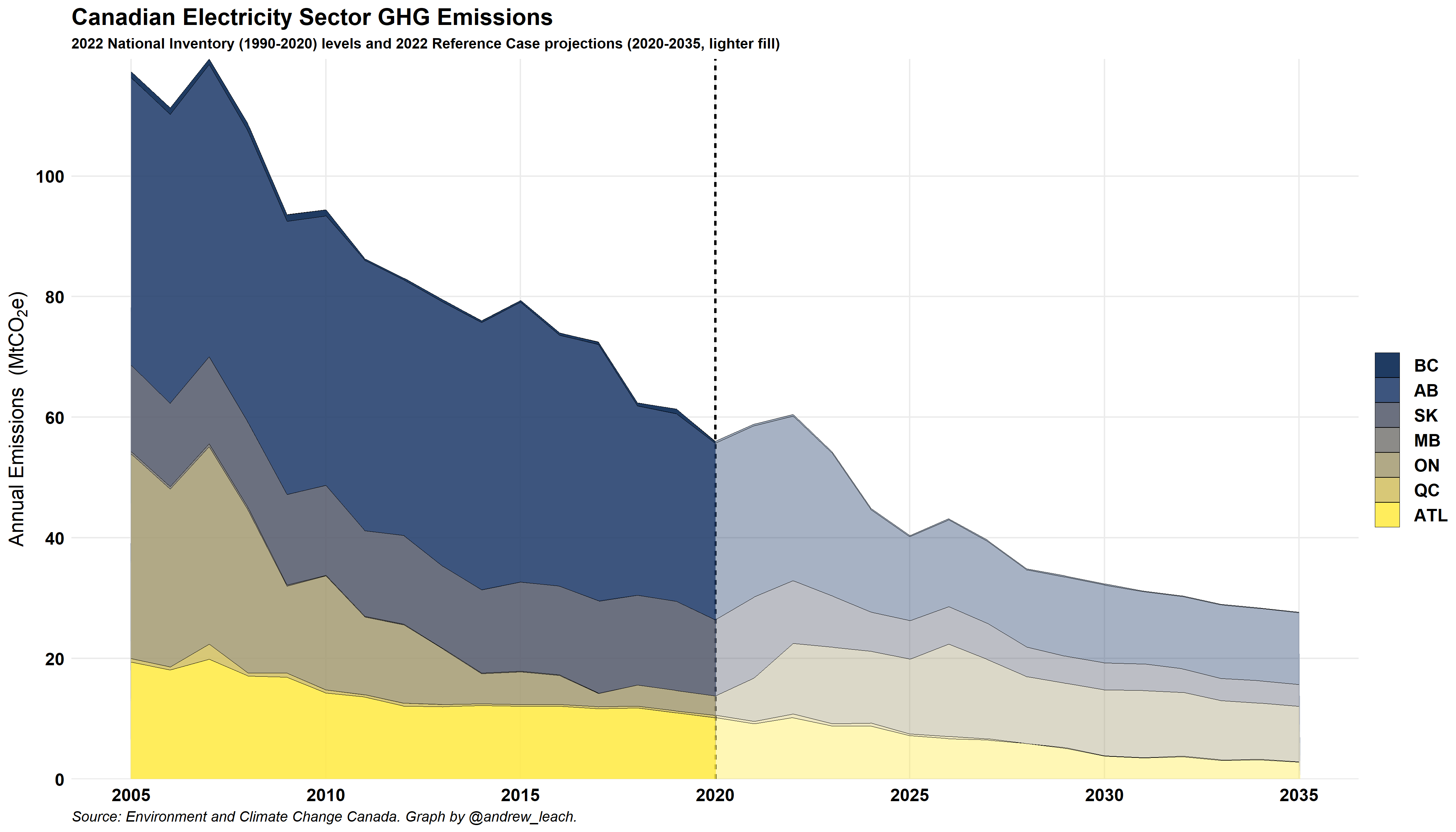
Second, I’d like you to produce a graph of the projections and emissions combined. You can choose whether to use the Reference Case or the Additional Measures Case, just make sure to label your graph appropriately. This is one of the more challenging graphs for this exercise. At a minimum, I’d like you to have a division line (use geom_vline()) to split between projections and inventory data: (2 marks)

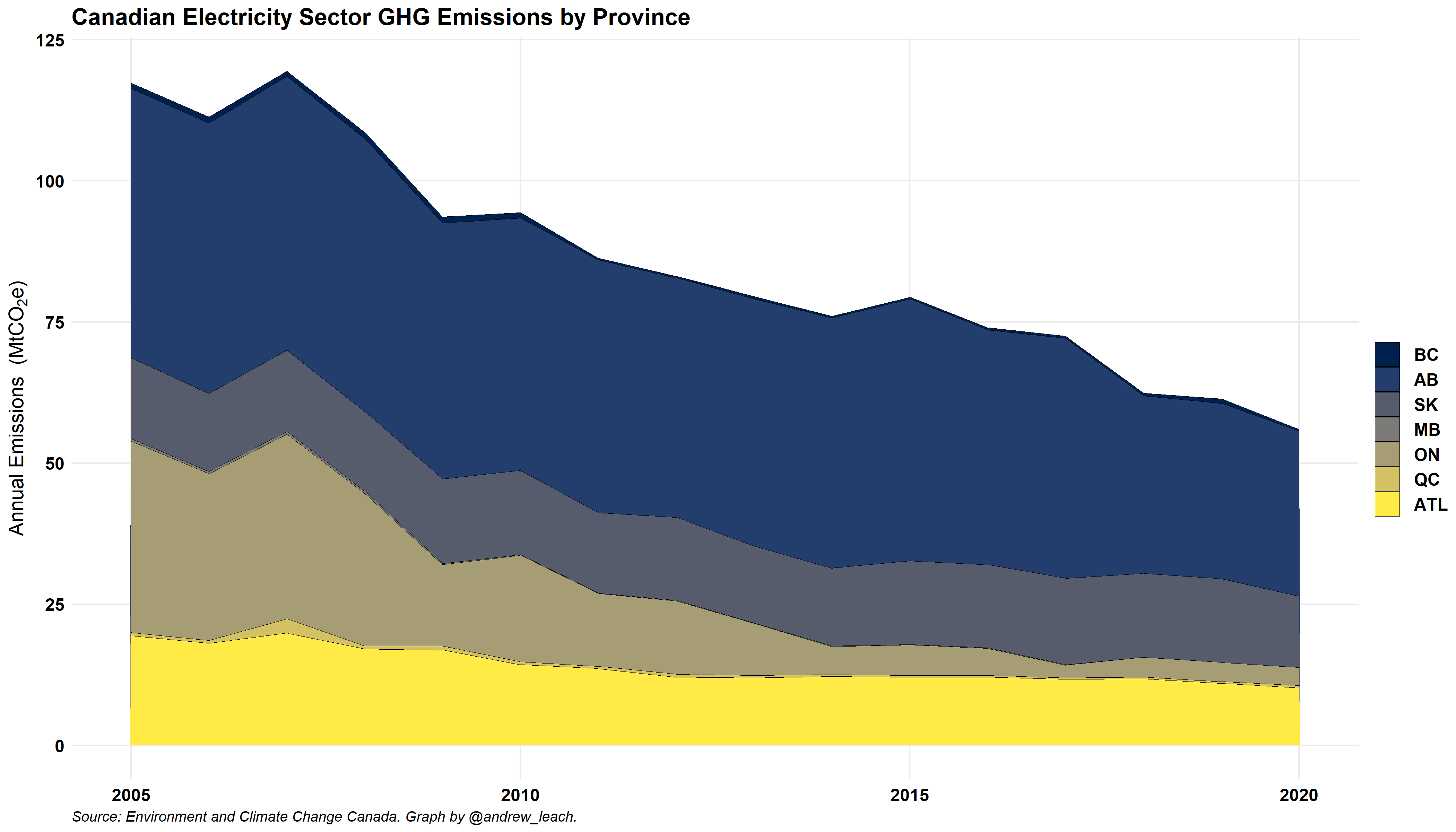
If you want to try to replicate mine with the more transparent fill for the projections, you can but you don’t have to do so.

If you want to try this, there are a number of ways to do this graph, but the most important thing to remember is that ggplot makes plots in layers, and this is basically a combination of two geom_area() plots (the projection, plot A, and the inventory, plot B) graphed one on top of the other with different transparency (alpha) values.

So, you need two geom_area() lines. For mine, I use something like this:

#start with the data filtered to include either the inventory for years up to 2020 and the projections for the later years
#I have a variable, project_case, that stores the name of the projection I am using
geom_area(aes(year,emissions,fill=prov),color="black",position = "stack",size=0.1,alpha=.4)+ #essentially plot A above
  geom_area(data=filter(proj_data,emissions>0 & scenario%in% c(inventory,project_case) & prov !="Canada" & year<=2020 & sector=="Electricity"),
            aes(year,emissions,fill=prov),color="black",position = "stack",size=0.1,alpha=.8)+ #the data in plot B above

If you get that to work, I’ll give you a bonus mark. (+ 1 Bonus)

Deliverable 4: The Merit Order (3 total marks)

In class, we’ve talked about the merit order, and so now is your chance to make a market supply curve with real data. I’ve extracted and processed some of the AESO merit order data for you here (merit_data.csv). This file contains over 35,000 observations detailing the market behaviour during the first of the grid alerts in January of 2024. Some of the variable names are self-explanatory, but here are the important details on what’s in the data:

date is obvious, and he is hour ending. So an observation for the hour 7pm to 8pm will have he=20.

Alberta market data on internal load (alberta_internal_load) and pool prices (pool_price) as you used in the AESO data exercise

import_export is equal to I if the offer in question is from imports

Plant characteristics AESO_Name and asset_id, Capacity in MW, Plant_Type and Plant_Fuel.

Offer characterisitcs: each plant may offer up to 7 blocks, indexed by block_number and each block has a price and the offer corresponds to a range of the plant’s capacity, from and to. So, the first 100MW of a 300MW plant would have block number 1 (0 is used if they only offer a single block), from=0, and to=100. The block size would be 100MW, the available_mw would also be 100MW. If it is dispatched, then dispatched=1 and if the full block is dispatched then dispatched_mw=100MW. A flexible block, indicated by flexible=1 may be partly dispatched, whereas an inflexible block is all-or-nothing

This is likely the most challenging graph I’ll ask you to make this term. So, before you get too frustrated with it, check out what it shows:

On Friday, Saturday, and Sunday, 7pm loads exceeded offered supply;

On Thursday (the record load day), the wind was much more of a factor than on the rest of the days and so the price wasn’t as high and there was no grid alert;

On each of Friday, Saturday, and Sunday, prices were at the $1000/MWh cap in the hour ended 7pm.

Now, for the hints. You’ll need them.

You’re going to want to filter your data to get rid of Jan. 10, 2024 and to keep the hours ending 7pm.
You need to create the x-axis variable (the cumulative offered supply). Here’s what I did: group_by(date)%>% arrange(price,Plant_Fuel)%>% mutate(merit=cumsum(size)%>%ungroup(). This will sort by offer price from low to high in blocks by Plant Type for each day, and then it will do a cumulative sum of offered blocks. merit is the x-axis variable in my graphs.
Use geom_rect(aes(xmin=merit-size,xmax=merit,ymin=-20,ymax=price,group=Plant_Fuel,fill=Plant_Fuel)) to create the blocks, and use geom_vlineandgeom_hline` to create the vertical and horizontal lines at pool prices and Alberta internal loads;
facet_wrap by date;
I made a date_string=as_factor(gsub(" 0", " ", format(date, "%A %B %d, %Y"))) which creates my formatted dates for the facet_wrap. You don’t need to do this but I think it looks cleaner.

You don’t have to replicate all the elements of my graph (legend colours, order, etc.). Just make a nice plot.

RMD File and HTML/PDF Preparation

As before, use the basic RMD file to complete this (and future) assignments, just rename it assignment 3. But, remember to clean up your HTML for deliverable 1!