Data Exercise, Week 1

BP Statistical Review of World Energy

This week, the first part of our Data Exercise focuses on an interesting source of data, the Statistical Review of World Energy, now published by the bp-affiliated Energy Institute. We’ll use this to learn a couple of new commands in R. The idea is to ramp you on-board with R slowly but surely, and this exercise is not graded. Later this month, you will have a graded exercise that uses some of these skills. For today, let’s make a graph of primary energy consumption by source.

The reason I wanted you to use this data this week is so that you can set yourself up in parallel in Excel and R so that you can visualize what’s happening in R behind the scenes and so that you can also get used to using spreadsheet-based data in R. You can do this exercise all in scripts, but I’d encourage you to build an RMarkdown document so that you get used to using them as you’ll need them for assignments later on. If you want to do so, then you can adapt all of these code chunks into your own R-Markdown (RMD) file, and you can use week2.Rmd as your starting point. Knit it before you start playing with it, just so you see that it works, then make a clean version to use for this week’s exercise.

There is also a lot of data cleaning to do, which will help you get your head around how data are stored in R.

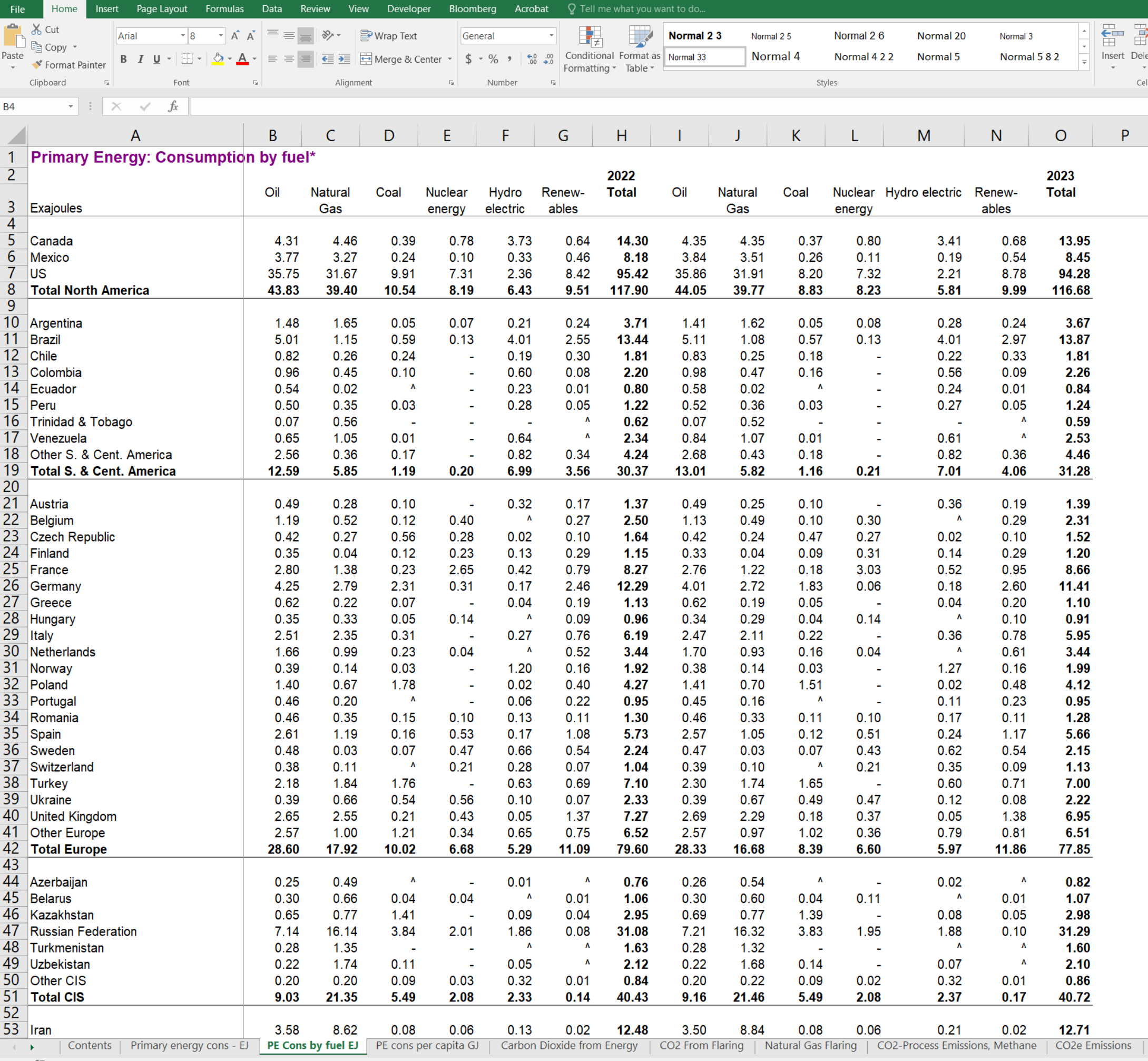
First, as you likely normally would, download the XLSX file for the Statistical Review. Open it in Excel or Sheets, whichever you normally use. For this exercise, we’re going to use the third tab, for Total Primary Energy Consumption By Fuel (labelled PE Cons by fuel EJ).

We’re going to learn about a few things here: reading from Excel using library(readxl) (make sure you have the library installed), more filtering skills, and making stacked bar charts. I’m going to use some kableExtra tables in this document just to make things a bit easier for you to see, but you don’t need to use those parts to make the graph at the end.

As usual, we’ll start with loading the packages we need. Create a code chunk in your document that looks like this:

library(tidyverse)
library(kableExtra)
library(readxl)
library(janitor)

Let’s download the data. Create a code chunk to do this and then to read it into R.

#check to see if the file exists. The first line after the if will only run if it doesn't
#you don't need this line, but it's a nice efficiency improvement for your code and one that I should use more often
if(!file.exists("bp_2024.xlsx"))
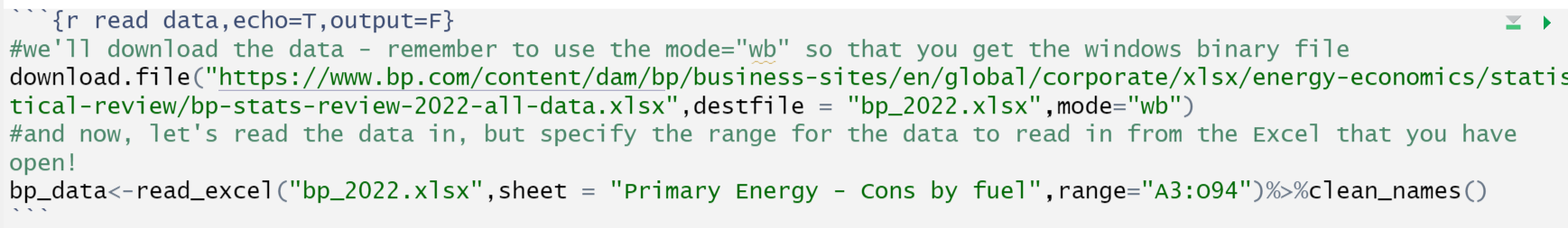
#we'll download the data giving it a local file name that's easy to deal with - remember to use the mode="wb" so that you get the windows binary file
    download.file("https://www.energyinst.org/__data/assets/excel_doc/0020/1540550/EI-Stats-Review-All-Data.xlsx",destfile = "bp_2024.xlsx",mode="wb")
#and now, let's read the data in, but specify the range for the data to read in from the Excel that you have open!
bp_data<-read_excel("bp_2024.xlsx",sheet = "PE Cons by fuel EJ",range="A3:O94")%>%clean_names()

Now’s the first lesson of the day: how to execute code chunks while working on your markdown document.

These parts are code chunks and you can execute them individually (you should start from the top and do them in sequence to make sure packages are loaded - by clicking that green triangle). You can also basically start over by clicking the grey triangle with the green bar, which will run all your code chunks from the start of your document. This is the equivalent to running the commands in sequence in a script.

Important note: running a code chunk is like running an R script or executing commands from the console. When you eventually go to knit your RMarkdown document, it is basically running in a new, clean environment, so it will re-do all the code chunks in sequence starting from scratch.

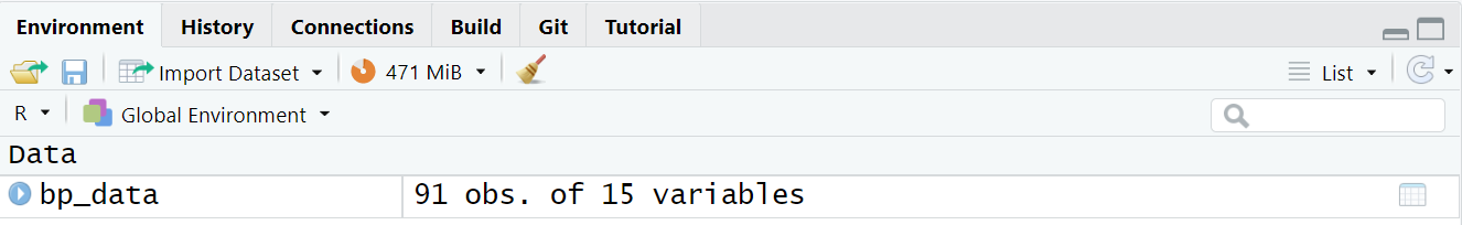
So, try it - copy and add the first two code chunks in this document to a new document of your own (or use the template) and, once you run then, you’ll see that you have the bp_data in memory. You can see that in the top right corner of your RStudio screen.

Click on it and you’ll open a viewer window and you’ll be able to see how R read in the data. It will look something like this:

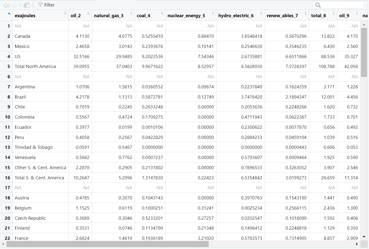
It’s ugly. But, you know what you’re dealing with. Let’s clean it up. In this case, it will be much easier for you to do while looking at the Excel as well.

First thing we know is that, for 2023 data, we only want columns 1 and 9-15 of the worksheet, so let’s do that using the select command.

#select is for picking columns. You can use it with numbers or names
#right now, our names aren't clear, so let's use numbers
bp_data<-bp_data %>% select(1,seq(9,15))

That gives us a much cleaner data set, but the names are all messed up. So, let’s fix them.

#assign new column names
names(bp_data)<-c("country","Oil","Natural Gas","Coal","Nuclear","Hydro","Renewables","Total")
#make sure they're "clean"
bp_data<-bp_data%>%clean_names()

So, now we have a much nicer data set, but there’s still the problem of all the blank rows. So, let’s clean that up too, using filter:

#remove observations that have an NA for country (ie. choose the ones that don't)
#this is going to annoy you, but ! is like "not" in this context.
bp_data<-bp_data%>%filter(!is.na(country))

If you mess code up at some point, you can always go back and re-read the data and start over, executing each of the chunks on the way back to here to make sure it works.

Now, I’m going to use a little bit of a fancier table maker to show you the data I’ve got after running all of this, using the kableExtra package:

  bp_data %>%
    kbl(escape = FALSE) %>%
    kable_styling(fixed_thead = T,bootstrap_options = c("hover", "condensed","responsive"))%>%
  scroll_box(width = "1000px", height = "400px")%>%
#adding this I() at the end of a chain of commands is like a placeholder in case you would otherwise end with a %>%. 
# It makes it easier to paste in code from elsewhere
      I()

country	oil	natural_gas	coal	nuclear	hydro	renewables	total
Canada	4.352	4.346	0.371	0.799	3.406	0.676	13.950
Mexico	3.837	3.513	0.264	0.111	0.191	0.537	8.453
US	35.858	31.913	8.197	7.324	2.210	8.779	94.281
Total North America	44.048	39.772	8.831	8.234	5.807	9.993	116.684
Argentina	1.409	1.618	0.046	0.080	0.280	0.238	3.671
Brazil	5.108	1.080	0.573	0.130	4.009	2.974	13.873
Chile	0.832	0.253	0.176	0.000	0.225	0.329	1.815
Colombia	0.977	0.470	0.156	0.000	0.560	0.093	2.255
Ecuador	0.579	0.018	0.002	0.000	0.237	0.007	0.844
Peru	0.519	0.364	0.029	0.000	0.272	0.054	1.238
Trinidad & Tobago	0.068	0.522	0.000	0.000	0.000	0.000	0.590
Venezuela	0.843	1.069	0.007	0.000	0.613	0.000	2.531
Other S. & Cent. America	2.676	0.430	0.176	0.000	0.819	0.359	4.459
Total S. & Cent. America	13.010	5.821	1.165	0.211	7.013	4.055	31.276
Austria	0.486	0.248	0.096	0.000	0.363	0.192	1.385
Belgium	1.134	0.493	0.099	0.295	0.004	0.286	2.311
Czech Republic	0.418	0.241	0.471	0.273	0.022	0.100	1.524
Finland	0.327	0.043	0.088	0.307	0.142	0.288	1.196
France	2.764	1.219	0.178	3.035	0.519	0.948	8.664
Germany	4.012	2.724	1.826	0.065	0.184	2.600	11.410
Greece	0.619	0.194	0.048	0.000	0.037	0.201	1.099
Hungary	0.337	0.295	0.036	0.143	0.002	0.098	0.911
Italy	2.473	2.110	0.217	0.000	0.364	0.782	5.945
Netherlands	1.703	0.928	0.158	0.036	0.001	0.611	3.436
Norway	0.385	0.137	0.035	0.000	1.273	0.163	1.991
Poland	1.405	0.705	1.506	0.000	0.022	0.478	4.116
Portugal	0.445	0.161	0.000	0.000	0.113	0.229	0.948
Romania	0.455	0.327	0.114	0.100	0.171	0.108	1.276
Spain	2.568	1.055	0.119	0.510	0.238	1.173	5.662
Sweden	0.466	0.026	0.065	0.435	0.618	0.542	2.151
Switzerland	0.387	0.099	0.004	0.209	0.346	0.088	1.133
Turkey	2.301	1.743	1.649	0.000	0.597	0.713	7.003
Ukraine	0.393	0.675	0.487	0.470	0.119	0.076	2.220
United Kingdom	2.688	2.286	0.184	0.366	0.049	1.378	6.950
Other Europe	2.566	0.973	1.015	0.360	0.791	0.808	6.513
Total Europe	28.333	16.681	8.395	6.604	5.973	11.860	77.846
Azerbaijan	0.257	0.544	0.000	0.000	0.016	0.003	0.820
Belarus	0.304	0.604	0.041	0.105	0.003	0.009	1.066
Kazakhstan	0.689	0.771	1.386	0.000	0.082	0.053	2.981
Russian Federation	7.212	16.321	3.834	1.951	1.878	0.095	31.291
Turkmenistan	0.279	1.323	0.000	0.000	0.000	0.000	1.602
Uzbekistan	0.222	1.677	0.137	0.000	0.065	0.003	2.104
Other CIS	0.199	0.215	0.089	0.024	0.321	0.010	0.857
Total CIS	9.161	21.457	5.486	2.080	2.366	0.172	40.722
Iran	3.502	8.840	0.079	0.060	0.212	0.020	12.712
Iraq	1.803	0.673	0.000	0.000	0.032	0.004	2.512
Israel	0.445	0.452	0.138	0.000	0.000	0.079	1.114
Kuwait	0.762	0.808	0.006	0.000	0.000	0.002	1.577
Oman	0.466	1.062	0.005	0.000	0.000	0.015	1.548
Qatar	0.613	1.591	0.000	0.000	0.000	0.014	2.218
Saudi Arabia	7.431	4.109	0.005	0.000	0.000	0.054	11.598
United Arab Emirates	2.204	2.408	0.102	0.290	0.000	0.129	5.133
Other Middle East	1.059	0.854	0.044	0.000	0.014	0.074	2.046
Total Middle East	18.285	20.798	0.379	0.349	0.258	0.390	40.459
Algeria	0.858	1.667	0.007	0.000	0.001	0.006	2.538
Egypt	1.494	2.162	0.050	0.000	0.129	0.103	3.938
Morocco	0.571	0.032	0.292	0.000	0.002	0.081	0.977
South Africa	1.086	0.171	3.325	0.080	0.016	0.175	4.853
Other Africa	4.484	2.133	0.408	0.000	1.364	0.174	8.564
Total Africa	8.492	6.164	4.082	0.080	1.512	0.539	20.869
Australia	2.166	1.444	1.508	0.000	0.143	0.759	6.021
Bangladesh	0.518	1.013	0.282	0.000	0.006	0.012	1.831
China	32.726	14.574	91.939	3.901	11.465	16.134	170.739
China Hong Kong SAR	0.574	0.174	0.147	0.000	0.000	0.008	0.903
India	10.573	2.254	21.981	0.433	1.395	2.380	39.016
Indonesia	3.096	1.636	4.320	0.000	0.230	0.826	10.108
Japan	6.655	3.327	4.536	0.695	0.697	1.493	17.404
Malaysia	1.787	1.659	0.983	0.000	0.295	0.085	4.807
New Zealand	0.319	0.137	0.041	0.000	0.248	0.116	0.861
Pakistan	0.782	1.362	0.617	0.201	0.350	0.060	3.372
Philippines	0.933	0.115	0.882	0.000	0.095	0.168	2.193
Singapore	2.994	0.444	0.014	0.000	0.000	0.018	3.470
South Korea	5.363	2.163	2.694	1.620	0.035	0.559	12.434
Sri Lanka	0.218	0.000	0.059	0.000	0.055	0.025	0.358
Taiwan	1.635	1.006	1.490	0.160	0.037	0.201	4.529
Thailand	2.311	1.698	0.605	0.000	0.062	0.331	5.007
Vietnam	1.195	0.260	2.323	0.000	0.757	0.356	4.891
Other Asia Pacific	1.256	0.407	1.274	0.000	0.855	0.037	3.829
Total Asia Pacific	75.102	33.674	135.695	7.009	16.723	23.571	291.774
Total World	196.430	144.366	164.034	24.567	39.651	50.580	619.629
of which: OECD	87.145	63.252	25.150	16.437	12.957	24.956	229.897
Non-OECD	109.285	81.114	138.884	8.130	26.694	25.625	389.732
European Union	21.446	11.501	5.483	5.559	3.046	9.349	56.383

I still don’t have exactly what I want, because I still have a lot of lines that don’t contain data I want to graph - I just want to use the totals, so I’ll show you a couple of tricks to clean those out.

#keep only observations that have total in the country cell using the grepl command
#grepl is a logical search function, so it will keep any observation (row) for which the term Total (case sensitive) appears in the country column
bp_data<-bp_data%>%filter(grepl("Total",country))

grepl is a really handy command that returns true for any cell that contains the word “Total” and false otherwise. It will be case sensitive, so check to make sure it worked. There are tricks to make it more general, but we’ll deal with those later.

Now, in this case, I want to make a graph by region, so I’m going to clean up the data a bit more. I’ll use gsub to find and replace text to strip the word “Total” out of all my regions.

#mutate to strip out the totals (note the space after total inside the quotes)
#gsub is a text substitution command, like a find and replace
bp_data<-bp_data%>%mutate(country=gsub("Total ","",country))

And now we have the data that we want to graph:

  bp_data %>%
    kbl(escape = FALSE) %>%
    kable_styling(fixed_thead = T,bootstrap_options = c("hover", "condensed","responsive"))%>%
  #scroll_box(width = "1000px", height = "400px")%>%
#adding this I() at the end of a chain of commands is like a placeholder in case you would otherwise end with a %>%. 
# It makes it easier to paste in code from elsewhere
      I()

country	oil	natural_gas	coal	nuclear	hydro	renewables	total
North America	44.05	39.77	8.831	8.234	5.807	9.993	116.7
S. & Cent. America	13.01	5.82	1.165	0.211	7.013	4.055	31.3
Europe	28.33	16.68	8.395	6.604	5.973	11.860	77.8
CIS	9.16	21.46	5.486	2.080	2.366	0.172	40.7
Middle East	18.29	20.80	0.379	0.349	0.258	0.390	40.5
Africa	8.49	6.16	4.082	0.080	1.512	0.539	20.9
Asia Pacific	75.10	33.67	135.695	7.009	16.723	23.571	291.8
World	196.43	144.37	164.034	24.567	39.651	50.580	619.6

This is going to be the part that you find counter-intuitive, and is one of the hardest things about graphing data in groups (or using flat data files), but there are going to be a lot of those in our future, so let’s learn about them.

To make this work well, we want to transform our data from wide, with the variables one in each column, to long with data stacked vertically and an indicator variable for the groupings we need. It’s easier to see than to describe, so let’s do it and then talk about it:

# we're going to pivot the data to a longer style, by country
# we're going to end up values going to a variable called tpes and names going to a variable called source
  bp_data<-bp_data%>%pivot_longer(-country,names_to = "source", values_to = "tpes")

#show me the data
bp_data %>%
    kbl(escape = FALSE) %>%
    kable_styling(fixed_thead = T,bootstrap_options = c("hover", "condensed","responsive"),full_width = T)%>%
  scroll_box(width = "1000px", height = "400px")%>%
#adding this I() at the end of a chain of commands is like a placeholder in case you would otherwise end with a %>%. 
# It makes it easier to paste in code from elsewhere
      I()

country	source	tpes
North America	oil	44.048
North America	natural_gas	39.772
North America	coal	8.831
North America	nuclear	8.234
North America	hydro	5.807
North America	renewables	9.993
North America	total	116.684
S. & Cent. America	oil	13.010
S. & Cent. America	natural_gas	5.821
S. & Cent. America	coal	1.165
S. & Cent. America	nuclear	0.211
S. & Cent. America	hydro	7.013
S. & Cent. America	renewables	4.055
S. & Cent. America	total	31.276
Europe	oil	28.333
Europe	natural_gas	16.681
Europe	coal	8.395
Europe	nuclear	6.604
Europe	hydro	5.973
Europe	renewables	11.860
Europe	total	77.846
CIS	oil	9.161
CIS	natural_gas	21.457
CIS	coal	5.486
CIS	nuclear	2.080
CIS	hydro	2.366
CIS	renewables	0.172
CIS	total	40.722
Middle East	oil	18.285
Middle East	natural_gas	20.798
Middle East	coal	0.379
Middle East	nuclear	0.349
Middle East	hydro	0.258
Middle East	renewables	0.390
Middle East	total	40.459
Africa	oil	8.492
Africa	natural_gas	6.164
Africa	coal	4.082
Africa	nuclear	0.080
Africa	hydro	1.512
Africa	renewables	0.539
Africa	total	20.869
Asia Pacific	oil	75.102
Asia Pacific	natural_gas	33.674
Asia Pacific	coal	135.695
Asia Pacific	nuclear	7.009
Asia Pacific	hydro	16.723
Asia Pacific	renewables	23.571
Asia Pacific	total	291.774
World	oil	196.430
World	natural_gas	144.366
World	coal	164.034
World	nuclear	24.567
World	hydro	39.651
World	renewables	50.580
World	total	619.629

You’re probably not used to seeing data presented this way, and it’s not as nice for table visuals, but it’s great for graphing.

Let me show you what I mean: let’s make a stacked bar plot of the individual constituents of primary energy consumption by region.

bp_data %>%
  #take out the global observations
  filter(country!="World")%>%
  #take out the total column
  filter(source!="total")%>%
  #send the data to ggplot
  ggplot()+ #make a graph
  # here, we are going to add a column "geom" to our graph
  # the data are country on the x axis and tpes on the y axis
  geom_col(aes(country,tpes,fill=source),color="black",linewidth=.25)#the color "black" are the "linewidth" describe the outlines between blocks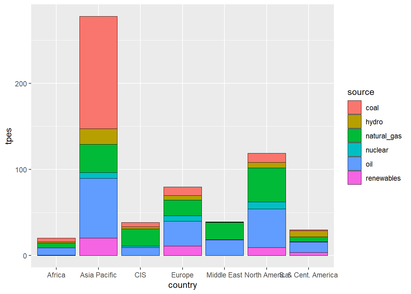

That’s a basic graph.

I think we might like to clean it up a bit, and get some colors to suit our sources a bit better. Let’s use a couple of other libraries, ggthemes and tools, so make sure you have those installed if you’re going to try to use them.

library(tools)
library(ggthemes)
bp_data %>%
  filter(country!="World")%>%
  filter(source!="total")%>%
  mutate(source=toTitleCase(gsub("_"," ",source)))%>% #strip out the underscore, convert to title case
  #take out the global observations and total column

  ggplot()+
  geom_col(aes(country,tpes,fill=source),color="black",linewidth=.25)+
  theme_economist_white()+#for fun, let's use the economist theme
  guides(fill=guide_legend(nrow = 1))+
  theme(legend.position = "bottom")+
  scale_fill_manual("",values=c("Coal"="black","Oil"="grey30","Natural Gas"="grey70","Nuclear"="orange","Hydro"="dodgerblue","Renewables"="darkgreen"))+
  theme(text = element_text(size=16))+
  labs(y="Primary Energy Consumption (Exajoules)",x="",
       title="Primary Energy Consumption by Region and Source, 2023",
       caption="Source: BP Statistical Review of World Energy")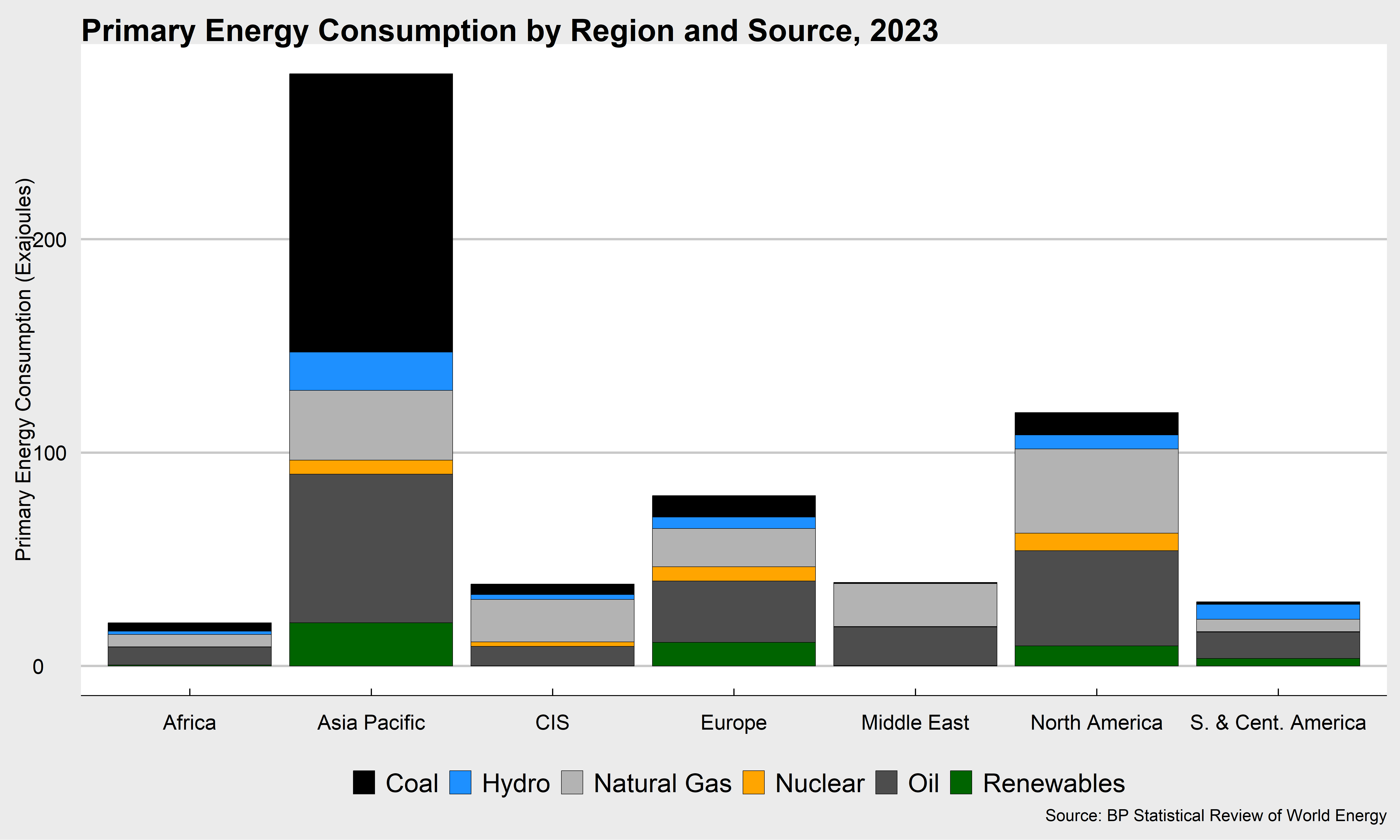

And, one of the frustrations in ggplot is that it assigns the variable groups as factors and, by default, they are sorted alphabetically. In this case, it doesn’t matter much, but just so you know what’s out there, let me show you one additional step which is to create your own factor for the sources of energy, and use the package forcats to reorder them. We’ll deal with these more in the future, so this is just a little added feature you might decide you need at some point.

library(forcats)
bp_data %>%
  filter(country!="World")%>%
  filter(source!="total")%>%
  mutate(source=toTitleCase(gsub("_"," ",source)))%>% #strip out the underscore, convert to title case
  mutate(source=as_factor(source))%>% #make the sources factors in the order they appear in the data
  mutate(source=fct_relevel(source,"Coal"))%>% #use fct-relevel to make coal the first factor level
  mutate(source=fct_rev(source))%>% #reverse the order
  #take out the global observations and total column

  ggplot()+
  geom_col(aes(country,tpes,fill=source),color="black",linewidth=.25)+
  theme_economist_white()+#for fun, let's use the economist theme
  guides(fill=guide_legend(nrow = 1))+
  theme(legend.position = "bottom")+
  scale_fill_manual("",values=c("Coal"="black","Oil"="grey30","Natural Gas"="grey70","Nuclear"="orange","Hydro"="dodgerblue","Renewables"="darkgreen"))+
  theme(text = element_text(size=16))+
  labs(y="Primary Energy Consumption (Exajoules)",x="",
       title="Primary Energy Consumption by Region and Source, 2023",
       caption="Source: BP Statistical Review of World Energy")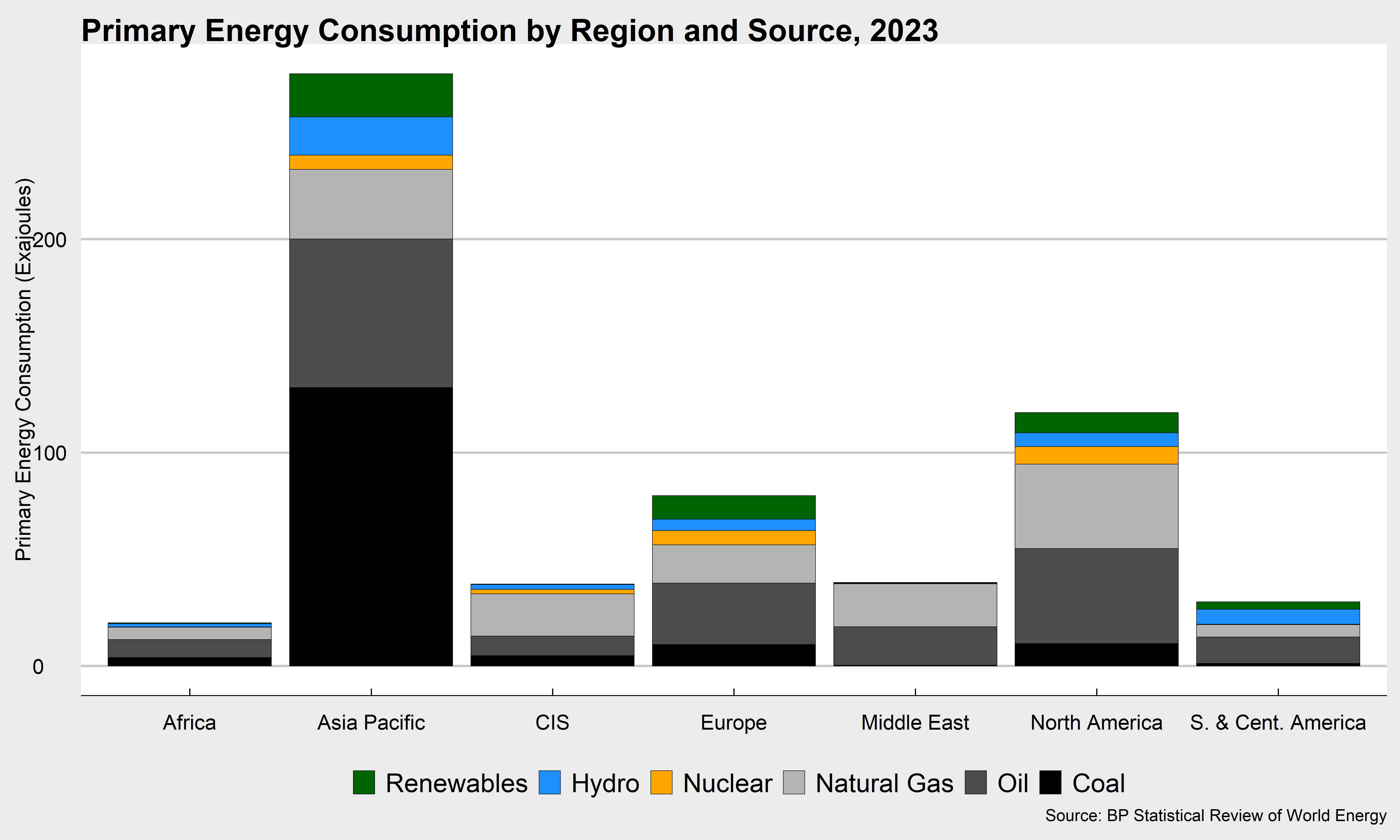

CANSIM and R for Statistics Canada Tables

I also wanted to quickly introduce to you the idea of specialized packages in R that make access to certain data repositories very easy. For this week, I’ll show you the cansim (or StatCan) data access package. Install the cansim package, and then let’s grab some energy supply data to make one of the graphs in the first sets of slides.

Table 25-10-0029-01 from Statistics Canada has Canadian primary energy supply data: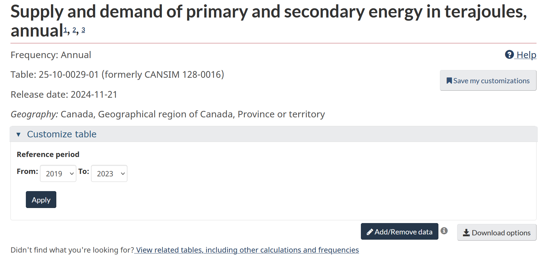

The nice thing about the r cansim package for R is that we can use it to download and process any of the data from those tables.

library(cansim)#load the cansim package
options(scipen = 999) #force it to use decimals not scientific notation
tpes_data<-get_cansim("25-10-0029-01")%>% clean_names()

This is quite a large set of data, going back to 1995 with a whole lot of different data points by energy source and region. We’re going to do a little bit of manipulation of the data to make a relatively simple graph of natural gas production, imports, and exports over time.

The first step is to modify the data using filter so that we get only the national data (geo==Canada) and for natural gas (fuel_type=="Natural gas") and we want only a select set of supply and demand charateristics (supply_and_demand_characteristics%in% c("Production","Exports","Imports")). Since the data are also provided for more than one unit of measurement, we also filter our to uom==Terajoules to leave us with only one. Here’s a nice example of how to use the filter command to pare down your data:

tpes_data<-tpes_data%>%
  filter(supply_and_demand_characteristics %in% c("Production","Exports","Imports"),
         geo=="Canada",
         fuel_type =="Natural gas",
         uom=="Terajoules")

and then we can make a graph:

 tpes_data %>% #pass the data to the graph
  ggplot(aes(ref_date,value/1000))+ #divide by 1000 to put it in petajoules
  #add lines for each group of data
  geom_line(aes(group=supply_and_demand_characteristics,color=supply_and_demand_characteristics),linewidth=1.25)+
  #create a colour scale
  scale_color_manual("",values=c("black","red","dodgerblue"))+
  labs(y="Primary Energy Production, Imports and Exports (PJ)", x="",
       title="Canadian Primary Energy Production, Imports, and Exports of Natural Gas")+
  scale_y_continuous(expand=c(0,0))+
  scale_x_discrete(expand=c(0,0))+
  expand_limits(y=0)+
  theme_classic()+
  NULL

We’ll likely use the cansim package a few more times this year, so make sure you’re familiar with it.

And, that’s this week’s data lesson. Try it out for yourself in your own document, using these code chunks as you see fit, to start to get ready for the first graded assignment later in the month.